Section 2.1 Points and Lines
Often, to get an idea of the behavior of an equation, we will make a picture that represents the solutions to the equations. A graph is simply a picture of the solutions to an equation. Before we spend much time on making a visual representation of an equation, we first have to understand the basis of graphing. Following is an example of what is called the coordinate plane.
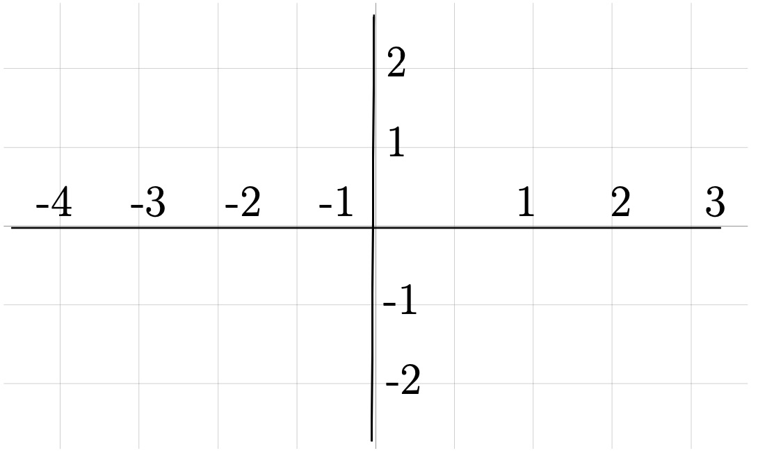
The plane is divided into four sections by a horizontal number line (\(x\)-axis) and a vertical number line (\(y\)-axis). Where the two lines meet in the center is called the origin. This center origin is where \(x = 0\) and \(y = 0\text{.}\) As we move to the right the numbers count up from zero, representing \(x=1, 2, 3\text{....}\)
To the left the numbers count down from zero, representing \(x = -1, -2, -3\text{....}\) Similarly, as we move up, the numbers count up from zero, \(y = 1, 2, 3\text{....,}\) and as we move down, count down from zero, \(y = -1, -2, -3\text{.}\) We can put dots on the graph which we will call points. Each point has an “address” that defines its location. The first number will be the value on the \(x\)-axis or horizontal number line. This is the distance the point moves left/right from the origin. The second number will represent the value on the \(y\)-axis or vertical number line. This is the distance the point moves up/down from the origin. The points are given as an ordered pair \((x, y)\text{.}\)
World View Note: Locations on the globe are given in the same manner, each number is a distance from a central point, the origin which is where the prime meridian and the equator. This “origin” is just off the western coast of Africa.
The following example finds the address or coordinate pair for each of several points on the coordinate plane.
Example 2.1.1.
Give the coordinates of each point.
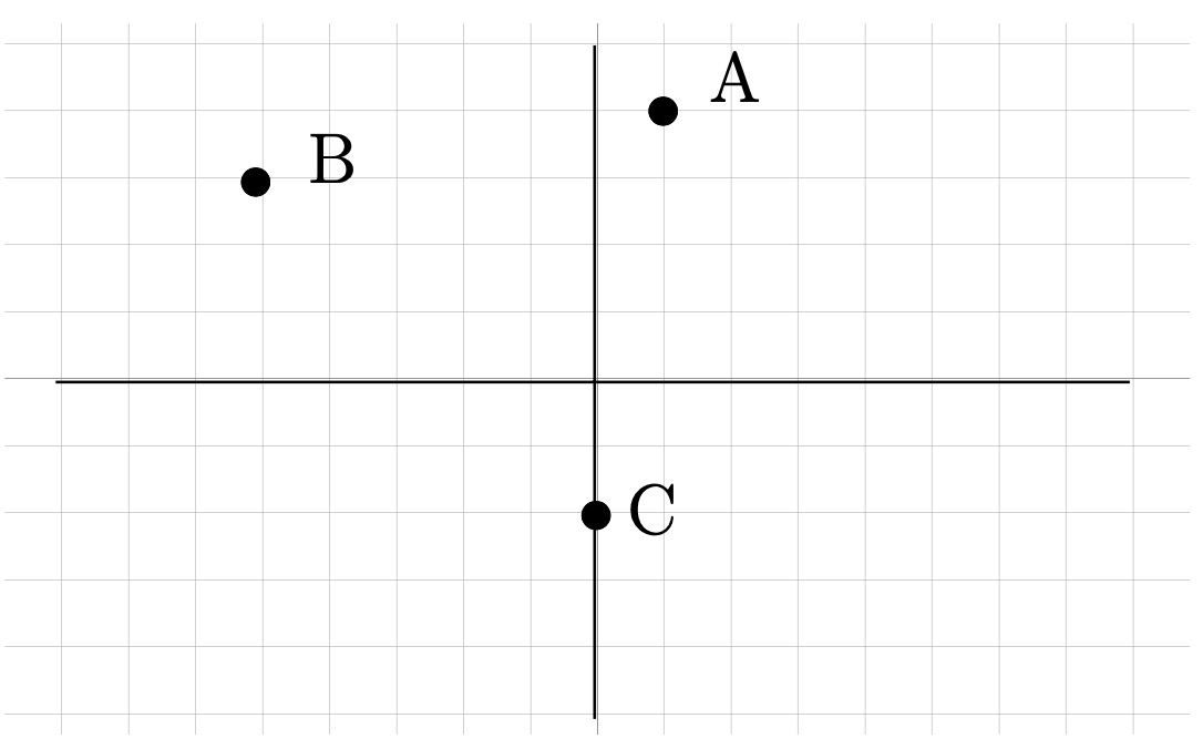
Tracing from the origin, point \(A\) is right \(1\text{,}\) up \(4\text{.}\) This becomes \(A(1, 4)\text{.}\) Point \(B\) is left \(5\text{,}\) up \(3\text{.}\) Left is backwards or negative, so we have \(B(-5, 3)\text{.}\) \(C\) is straight down \(2\) units. There is no left or right. This means we go right zero, so the point is \(C(0,-2)\text{.}\)
Just as we can give the coordinates for a set of points, we can take a set of points and plot them on the plane.
Example 2.1.2.
Graph the points \(A(3, 2)\text{,}\) \(B(-2, 1)\text{,}\) \(C(3, -4)\text{,}\) \(D(-2, -3)\text{,}\) \(E(-3, 0)\text{,}\) \(F(0, 2)\text{,}\) \(G(0, 0) \text{.}\)
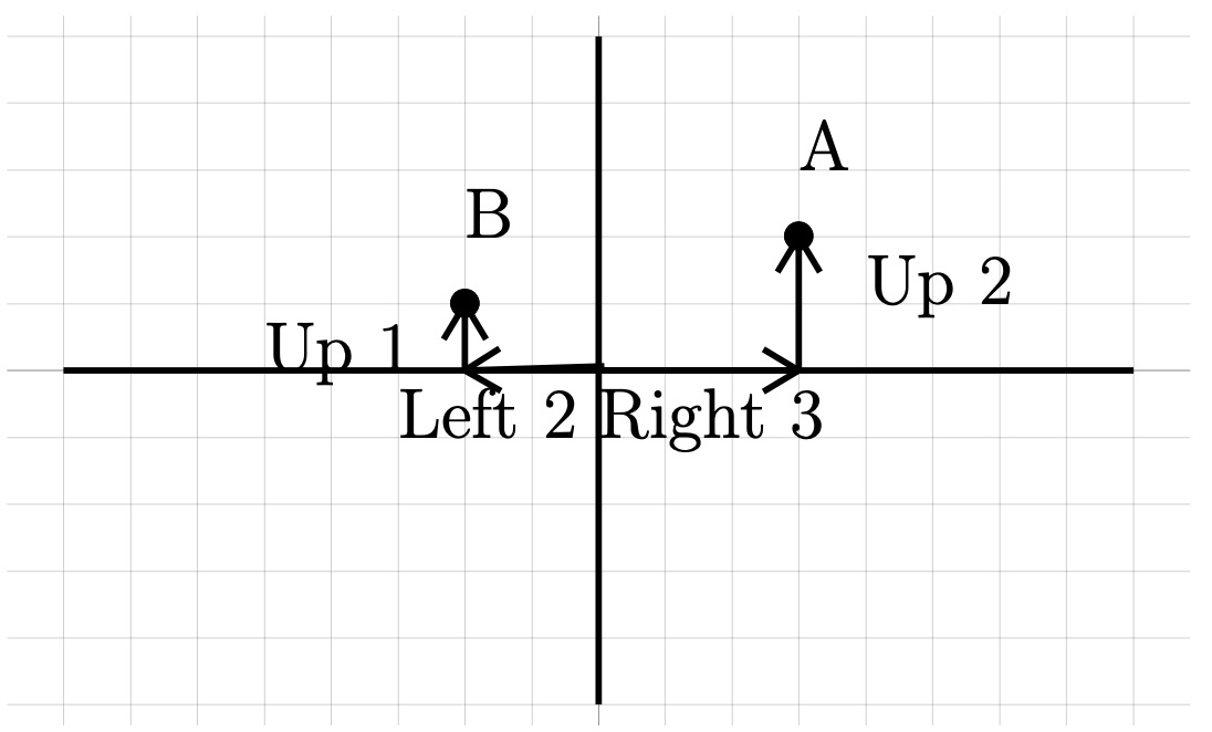
The first point, \(A\text{,}\) is at \((3, 2) \) this means \(x=3\) (right \(3\)) and \(y =2\) (up \(2\)). Following these instructions, starting from the origin, we get our point.
The second point, \(B(-2, 1) \text{,}\) is left \(2\) (negative moves backwards), up \(1\text{.}\) This is also illustrated on the graph.
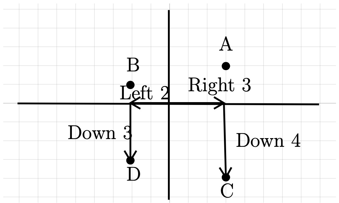
The third point, \(C (3, -4)\) is right \(3\text{,}\) down \(4\) (negative moves backwards).
The fourth point, \(D (-2, -3) \) is left \(2\text{,}\) down \(3\) (both negative, both move backwards).
The last three points have zeros in them. We still treat these points just like the other points. If there is a zero, there is just no movement.
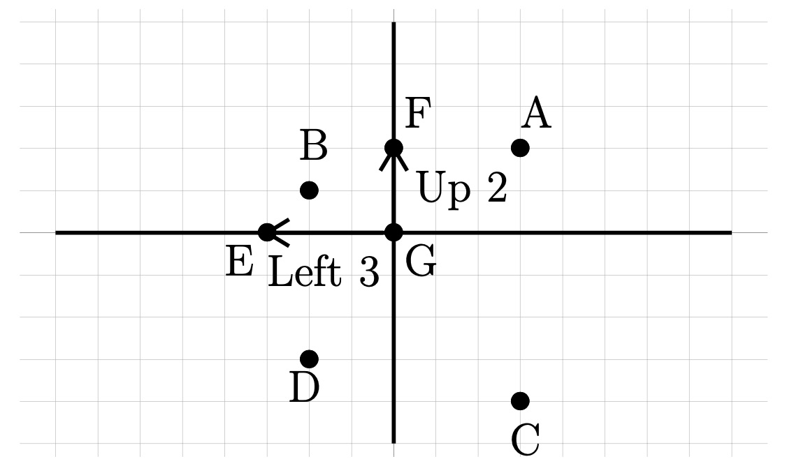
Next is \(E(-3, 0)\text{.}\) This is left \(3\) (negative is backwards), and up zero, right on the \(x\)-axis.
Then is \(F (0, 2)\text{.}\) This is right zero, and up two, right on the \(y\)-axis.
Finally is \(G(0, 0)\text{.}\) This point has no movement. Thus, the point is right on the origin.
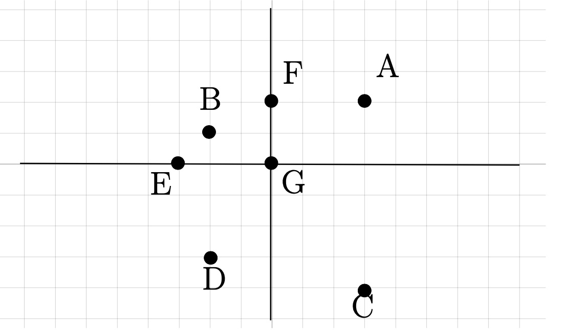
Our Solution
The main purpose of graphs is not to plot random points, but rather to give a picture of the solutions to an equation. We may have an equation such as \(y = 2x - 3\text{.}\) We may be interested in what type of solution are possible in this equation. We can visualize the solution by making a graph of possible \(x\) and \(y\) combinations that make this equation a true statement. We will have to start by finding possible \(x\) and \(y\) combinations. We will do this using a table of values.
Example 2.1.3.
Graph \(y=2x-3\)
We make a table of values
| \(x\) | \(y\) |
| \(-1\) | |
| \(0\) | |
| \(1\) |
We will test three values for \(x\text{.}\) Any three can be used.
| \(x\) | \(y\) |
| \(-1\) | \(-5\) |
| \(0\) | \(-3\) |
| \(1\) | \(-1\) |
Evaluate each by replacing \(x\) with the given value:
\(x=-1\text{;}\) \(y =2(-1)-3=-2-3=-5\)
\(x=0\text{;}\) \(y =2(0)-3=0-3=-3\)
\(x=1\text{;}\) \(y =2(1)-3=2-3=-1\)
\((-1, -5), (0, -3), (1, -1) \)
These then become the points to graph on our equation.
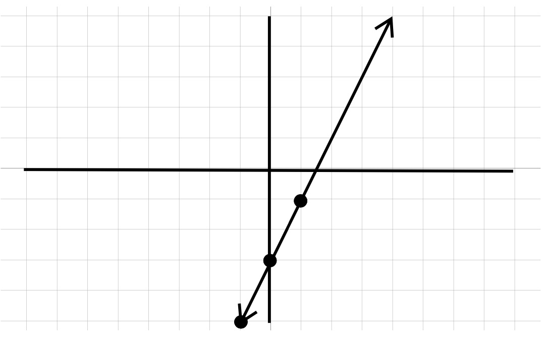
Plot each point.
Once the points are on the graph, connect the dots to make a line.
The graph is our solution.
What this line tells us is that any point on the line will work in the equation \(y = 2x-3\text{.}\) For example, notice the graph also goes through the point \((2, 1)\text{.}\) If we use \(x=2\text{,}\) we should get \(y =1\text{.}\) Sure enough, \(y =2(2)-3=4-3=1\text{,}\) just as the graph suggests. Thus, we have the line is a picture of all the solutions for \(y = 2x-3\text{.}\) We can use this table of values method to draw a graph of any linear equation.
Example 2.1.4.
| \(x\) | \(y\) |
| \(-3\) | |
| \(0\) | |
| \(3\) |
We will test three values for \(x\text{.}\) Any three can be used.
| \(x\) | \(y\) |
| \(-3\) | \(-4\) |
| \(0\) | \(-2\) |
| \(3\) | \(0\) |
Our completed table.
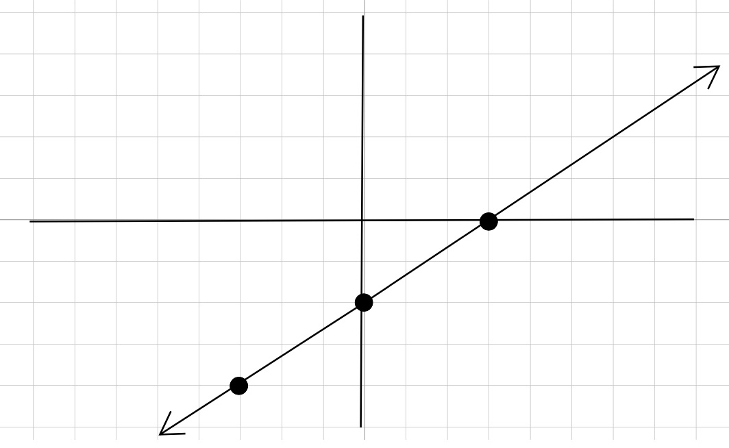
Graph points and connect dots
Our Solution
Exercises Exercises - Points and Lines
1.
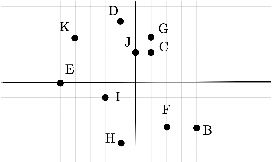
State the coordinates of each point.
2.
Plot each point.
\(L(-5, 5)\text{,}\) \(K(1, 0)\text{,}\) \(J(-3, 4)\text{,}\) \(I(-3, 0)\text{,}\) \(H(-4, 2)\) \(G(4,-2) \text{,}\) \(F(-2,-2)\text{,}\) \(E (3,-2)\text{,}\) \(D(0, 3)\text{,}\) \(C(0, 4)\text{,}\)
Exercise Group.
Sketch the graph of each line.
3.
\(y=-\frac{1}{4}x-3 \)
4.
\(y=x-1 \)
5.
\(y=-\frac{5}{4}x-4 \)
6.
\(y=-\frac{3}{5}x+1 \)
7.
\(y=-4x+2 \)
8.
\(y=\frac{5}{3}x+4 \)
9.
\(y=\frac{3}{2}x-5 \)
10.
\(y=-x-2 \)
11.
\(y=-\frac{4}{5}x-3 \)
12.
\(y=\frac{1}{2}x \)
13.
\(x+5y=-15 \)
14.
\(8x-y=5 \)
15.
\(4x+y=5 \)
16.
\(3x+4y=16 \)
17.
\(2x-y=2 \)
18.
\(7x+3y=-12 \)
19.
\(x+y=-1 \)
20.
\(3x+4y=8 \)
21.
\(x-y=-3 \)
22.
\(9x-y=-4 \)